A version of this project appears in Make: Robotic Arms

As a makerspace manager, one of the absolute best parts of my job is helping my students design their own custom robotics projects. Over the years, I began to realize that while most of my students were excited to learn the basics, there were some more advanced robotics tools that they assumed were way over their heads! This was especially true when it came to integrating and calculating the forward and inverse kinematics in their projects. This led me to develop a series of makerspace workshops with a simple goal: demystifying inverse kinematics! Whether you’re working on animatronics, humanoid or quadruped robots, or even a robotic arm project, inverse kinematics can help take all kinds of fun projects to the next level. Even better, getting started is easier than you might think!

When it comes to programming devices like servo motors with a microcontroller, getting that motor to move to a specific position is pretty easy! A few lines of code, some wires, and you’re done!

But what if you’re working on something like a robotic arm project? What if we needed the end of our robotic arm to move to a very specific location? We could certainly slowly figure out what angles we would need from all of our motors through trial and error, but that could take quite a while. That’s where inverse kinematics comes in! With just a little bit of math, we can write a program that will allow us to use any coordinate point we want as an input, and our code will calculate the exact angles our motors need to move to in order to move the end of our robotic arm to our goal coordinate.

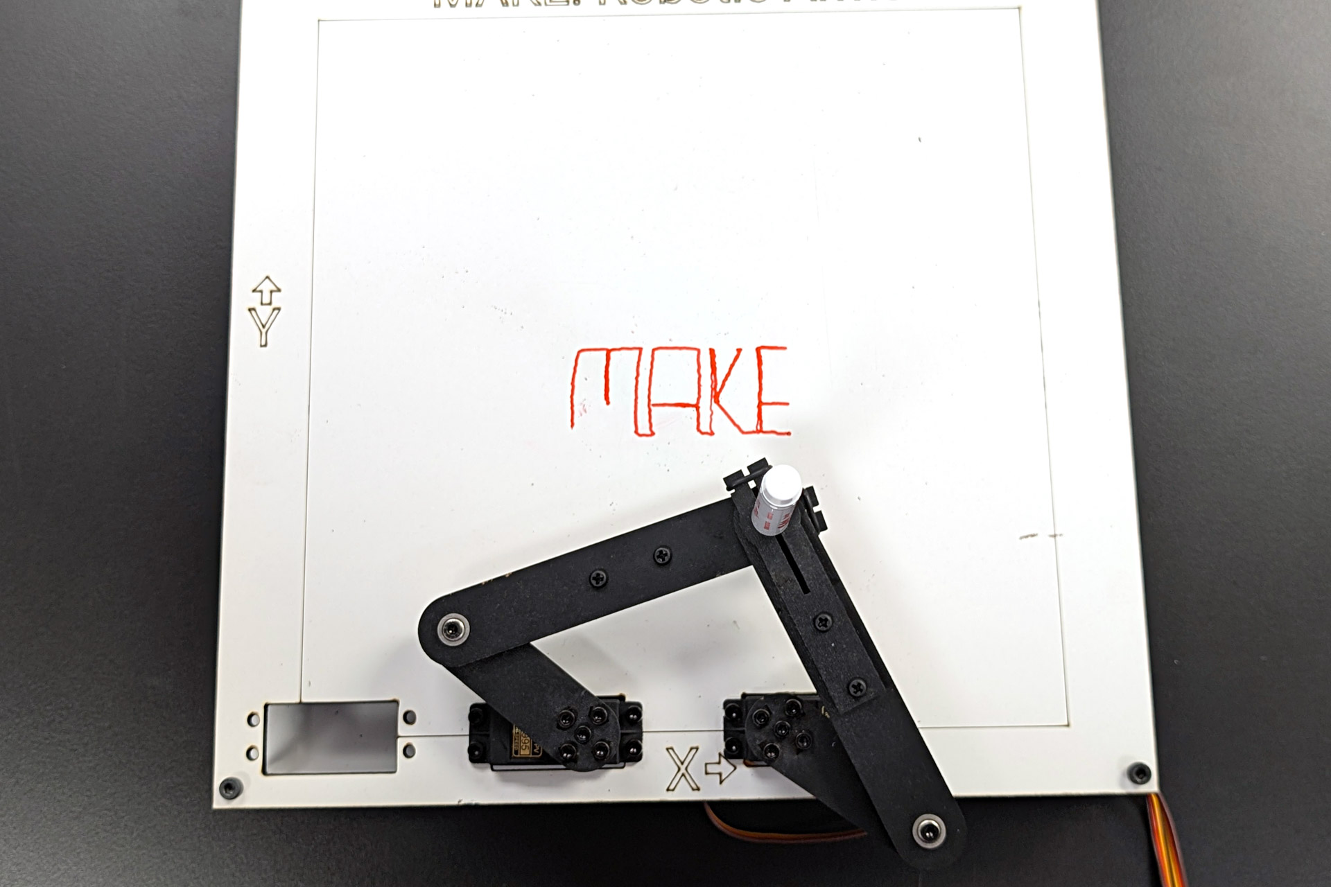
Once we have a robot that can move anywhere we want quickly and accurately, there are all kinds of fun things we can build, like building the legs of a robotic dog, the arms of a humanoid or an animatronics robotics project, and even building a DIY draw bot. In fact, that’s the goal of this article! We’re going to start by assembling a four-link robotic arm that will serve as the structure of our robot. Then we’ll take a look at a little math we’ll need in order to develop our inverse kinematics equations, and then we will put it all together to make a fun drawing robot!

One quick note, there are many different ways to build a drawing robot, and there may be more efficient methods out there, such as the linear assemblies found in devices like laser cutters and 3D printers. This project is much more about understanding the relationship between inverse kinematics and robotic joints and links to build a fun robotic arm project, as opposed to simply achieving the highest possible accuracy.

Ok, let’s get building!

What will the next generation of Make: look like? We’re inviting you to shape the future by investing in Make:. By becoming an investor, you help decide what’s next. The future of Make: is in your hands. Learn More.

Project Steps

Assembly Step 1

Download the .DXF files from the GitHub repository, and cut the files using whatever sort of CNC machine you would like. I recommend using a laser cutter, but the files could absolutely be imported into your favorite CAD program and converted for 3D printing. The base of the project and the links were designed to be laser cut directly out of whiteboard material to save costs, but almost any material will work with a little customization. General-purpose whiteboard sheets and acrylic sheets can be found online and even in your local Lowe’s or Home Depot. Once you have the base and top plate cut, we can begin the assembly!

Assembly Step 2

Using eight M3 x 10mm bolts and four M3 x 25mm standoffs, connect the base and top plate.

Assembly Step 3

Once the base is built, take two MG995 servos and bolt them to the base as shown. Make sure that the output shafts are in the exact orientation shown. Next, place two round metal servo horns on the two servos.

Assembly Step 4

Now that both motors are mounted, we can wire up and program our motors to move to a specific starting position. Because our goal is to develop the inverse kinematics for this system, having a set starting position is incredibly important. For this project, I will be using an Arduino Uno, but any microcontroller will work just fine. The wiring diagram for the project can be found below.

The red wires of both servos will be connected to the positive rail on the breadboard; the black wires should be connected to the negative rail. The yellow wire for servo one should be connected to digital pin 3, and similarly, the yellow wire for servo two should be connected to digital pin 5. Next, a single wire needs to be connected from a GND pin on the Arduino to the negative rail on the breadboard. Lastly, the positive and negative rails of the breadboard should be connected to the 5V 2A power supply.

Assembly Step 5

Once the circuit is wired up, we can write a quick Arduino sketch to set both of our servos to a starting position. In this case, we want both motors to have an angle of 90 degrees.

#include <Servo.h>
Servo servoOne;
Servo servoTwo;

void setup() {
     servoOne.attach(3);
     servoTwo.attach(5);
}

void loop() {
     servoOne.write(90);
     servoTwo.write(90);
}

Assembly Step 6

We can now attach the first two links to our newly programmed servos. Taking ten M3 x 5mm bolts, attach both links to the two servos.

Assembly Step 7

Next, we need to connect the second links for our two servos. Starting with the servo on the left, we will need one M3 x 20mm bolt, two 8mm bearings (size F693ZZ), one M3 x 3mm spacer, and one M3 locknut. Place the 8mm bearings through both links, the spacer in between both, and bolt both links together.

The second link for our second servo will be connected the exact same way but without the need for the 3mm spacer. When both links are connected, your project should look just like the image.

Assembly Step 8

Our final step will be bolting on the pen holders, and attaching our whiteboard marker! For our last step, we will need one thin whiteboard marker and two 8mm ID O-rings. The marker will be placed through the center hole shared by both of our second links, and the two O-rings will be placed on the ends of the top and bottom pen holder brackets.

Our final full assembly can be seen below.

Part Two: The Inverse Kinematics!

Before we write the code that will make all this possible, we need to determine our inverse-kinematics calculations. But first, we need to develop a more mathematical way of describing what’s going on with our robotic arm.

In the diagram, we can see something that looks a lot like our project, but we’ve added a coordinate system and given variables to the lengths of the links of our robotic arm as well as the angles of our actuators, the servomotors. We have also added two theoretical lines. Here, the lines c and e will help us create some triangles within our existing variables that will make our final calculations much easier down the road. Another added benefit of creating these two theoretical lines is the ability to create sub-angles. With this current setup, we have two sub-variables for each of our main variables.

Just as before, our goals for developing the inverse kinematics equations for our four-link system are to have the ability to provide our desired x and y coordinates for the end effector, our drawing pen, and have our equations calculate the actuator angles required to get there.

Calculating c and e

Our first step in finding the inverse kinematics will be to discover the value of our two theoretical line variables, c and e. Thankfully, this is a snap. All we’ll need is the Pythagorean theorem:

The Pythagorean theorem, which was very helpful in calculating the inverse kinematics of our first robotic arm, is a great tool for finding the lengths of a right triangle. Thankfully, our c and e variables create two simple right triangles within our systems.

We can think of the lines that make up our c and e variables as nothing more than the hypotenuse sides of two right triangles.

Think of these two lines as parts of a triangle that give us two nice and simple equations for determining the value of our c and e variables. Because two of the sides of our right triangle are equal to our value for x and y, finding the value of c is really easy. Finding the value of e is also pretty straightforward—the height of the second right triangle is the same, so we keep the y value. The length of the base of the second right triangle is equal to the length of the two triangles put together, d, minus the value of x. In our first example, things are nice and symmetrical, but this isn’t always the case.

Calculating b2 and a1

Now that we have the values of our c and e variables, we can start to solve for our angle variables. We’ll begin by solving our innermost angle variables, β2 and α1. Because these two sub-angles are also a part of the right triangles we’ve been working with, we can find their value easily using arctan.

Calculating b1 and a2

Now that we have our first set of sub-angle variables, our next step will be to calculate our next two sub-angle variables, β1 and α2. If we look back at our original diagram, these two angles are not a part of the right triangles we have been working with. They are angles within the non–right triangle portions of our diagram. Thankfully, if we recall the law of cosines, we know we can easily find the value of one of the angles in a non–right triangle as long as we know the length of every side of our triangle. If we were to isolate just the two non–right triangles, we see that we do in fact know the length of all three sides of the two non–right triangles.

One side of each of the triangles is made up of our c and e variables, and the other two sides of both triangles are made up of the length of our links. This means we can easily find the value of our two variables by plugging them into our law-of-cosines equation arccos.

Calculating Our Final b and a Values

Our final step is combining our sets of sub-angles into our final angle values. The main goal of our calculations is to find the final two angle values we can send to the actuators of our motors that will move our end effector into the position we need it to be. In our first example, this was a matter of simple addition. With our four-link system, however, things get a little more complicated. Our final β and α values will depend on the value of our x variable. In some cases, the position of the end effector in the x direction means we will need slightly different calculations to find our final angle values.

The final calculations will depend on whether the x value lies within the boundaries of the length between our two motors, otherwise known as our d value.

If x is less than 0:

If x is between 0 and d:

If x is greater than d:

With that, we have completed our final calculations! We now have everything we need to determine the inverse kinematics of our four-link system. Now that we know all our calculations, we can begin converting our inverse kinematics equations into code.

Part Three: The Code!

Let’s take another look at our circuit and add a useful component that will allow us to quickly and easily control the value of our goal coordinate for our project: a joystick! We can use the up-down axis of the joystick to increase and decrease the value of our y variable, which moves our robot up and down, and use the left-right axis of the joystick to increase and decrease the value of our x variable, moving our robot from left to right.

Connect the positive voltage pin of the joystick to the 5V pin on the Arduino, through the power rails of the breadboard. Connect the GND pin to the GND rail of the breadboard, and the x and y pins of the joystick to the A0 and A1 pins on the Arduino.

Now that we have wired all the components we’ll need, the final step will be converting our inverse kinematics equations into code and adding in the few lines we need to read our joystick values! Thankfully, Arduinos are great at math and have functions for each of the mathematical operations we’ll need to complete the calculations built into the programming language.

#include "Servo.h"
Servo servoOne;
Servo servoTwo;
//Setting up our IK variables
double x = 30.0;
double y = 120.0;
double linkOne = 100.0;
double linkTwo = 100.0;
double alphaOne;
double alphaTwo;
double alphaFinal;
double betaOne;
double betaTwo;
double betaFinal;
double c;
double d = 60.0;
double e;
int xval;
int yval;

void setup() {
  Serial.begin(9600);
  servoOne.attach(3);
  servoTwo.attach(5);
}

void loop()
{
  //IK Calculations
  yval = analogRead(A0);
  xval = analogRead(A1);
  c = sqrt((x*x)+(y*y));
  e = sqrt(((d-x)*(d-x))+(y*y));
  alphaOne = atan(y/x) * (180/PI);
  alphaTwo = acos(((linkTwo*linkTwo)-(c*c)-(linkOne*linkOne))
            /(-2*linkOne*c)) * (180/PI);
  betaOne = atan(y/(d-x)) * (180/PI);
  betaTwo = acos(((linkTwo*linkTwo)-(e*e)-(linkOne*linkOne))
            /(-2*linkOne*e)) * (180/PI);
  if(x < 0){ alphaFinal = 180 + ((alphaOne) + (alphaTwo)); betaFinal = 180 - ((betaOne) + (betaTwo)); } else if(x > d){
      alphaFinal = ((alphaOne) + (alphaTwo));
      betaFinal = -1 * ((betaOne) + (betaTwo));
    }
  else{
      alphaFinal = ((alphaOne) + (alphaTwo));
      betaFinal = 180 - ((betaOne) + (betaTwo));
    }

  //Printing the results! 
  Serial.print("alpha One: ");
  Serial.print(alphaOne);
  Serial.print(" beta One:");
  Serial.print(betaOne);
  Serial.print(" alpha Two: ");
  Serial.print(alphaTwo);
  Serial.print(" beta Two:");
  Serial.print(betaTwo);
  Serial.print(" Alpha: ");
  Serial.print(alphaFinal);
  Serial.print(" Beta: ");
  Serial.println(betaFinal);
  servoOne.write(alphaFinal);
  servoTwo.write(betaFinal);

/*
Depending on your customization, it may be a good idea to add some limits here! If you see your arms acting squirrely, add a statement  such as “if(xVal > 800 && xVal < 200)” */ if(xval > 800){
    x-=5;
  }
  if(xval < 300){ x+=5; } if(yval > 800){
    y-=5;
  }
  if(yval < 300){
    y+=5;
  }
}

Let’s break down the code we just sent over to our Arduino. One of the first things our code accomplishes is creating variables for our goal position on our grid in the form of a set of x and y coordinates. In this case, the coordinates (30, 120) were chosen so that the robot begins in the center of the grid. These values can be changed to have the pen start anywhere on the grid you’d like! Next, we can create the rest of the variables we need for our calculations. Each step of the equations has its own variable within the code.

The variables linkOne and linkTwo represent the lengths of the links in our system, which are both 100 mm. Next, the variables alphaOne, alphaTwo, alphaFinal, betaOne, betaTwo, and betaFinal represent all our sub-angle and final-angle variables. Lastly, the c and e variables are our theoretical triangle lines, and d represents the distance between the shafts of our two actuators.

Now that we have all the necessary variables, we can begin converting our inverse-kinematics equations into code. Though these lines of code might look much more complicated than some of our previous lines of code, if you go through them step by step, you’ll see that we’re taking each action we developed in our equations and converting it into code our Arduino can understand.

Once we have values for all our variables and have completed our main calculations, all that’s left is to combine our sub-angle variables into final-angle variables that will be sent to our actuators. As you may recall from our previous calculations, some of our final-angle calculations are dependent on the value of our x variable. Thankfully, three sets of conditional statements are all we need to make sure our angles are being calculated correctly, no matter what x and y values are chosen.

Conclusion

Part Four: Conclusion and Next Steps!

With that, our project is complete! As you move the joystick left and right, the pen should move from side to side, and as you move the joystick up and down, the pen should follow! This is a relatively simple first step, and one of the most exciting things about a project like this is all of the amazing ways in which it can be added to and customized! Some potential improvements and enhancements include:

  • Adding in a pen lift mechanism: One of the biggest potential areas of improvement would be adding a simple pen lift mechanism. With a few lines of code, the click button on the joystick could be used to trigger the lifting and lowering of the pen.
  • Swapping the servos for Stepper Motors: While servos are a great starting point, moving to more powerful and accurate stepper motors can significantly improve the precision and performance of the drawing robot.
  • Utilizing the “ServoEasing” library: The GitHub repo for this project has some really fun examples that take things a little further than what we cover in this article, such as incorporating the ServoEasing library, which allows for much smoother motions than the standard servo library. This ends up making the servos behave much more like a stepper motor would when using something like the popular accelstepper library. The servoEasing library was used in the sketch written to draw the “Make” logo seen in some of the project images.
  • Learning Linear Algebra: While this project uses basic geometry and trigonometry, diving into linear algebra is crucial for developing the inverse kinematics of more complex 3D robotic arms. This knowledge will be a great asset for future robotics projects.
  • Take a look at my Make:Book: This project was inspired by a book I wrote for Make, titled Make: Robotic Arms. In it, I detail step-by-step guides for building three exciting robotic arms, starting with simple 2D robots, all the way up to three-link 3D robotic arms! Each chapter introduces step-by-step guides to building the robots, the inverse kinematics equations for the projects, and fun sensors and methods of input for controlling the projects!

Images by Matt Eaton

A version of this project appears in Make: Robotic Arms, available for pre-order now.